Understanding the Concept of Statistics Through Examples

Library loading and functions

• Python libraries and functions are loaded before the tutorial.

from scipy import stats
import numpy as np
import matplotlib.pyplot as plt
import seaborn as sns

def generate_random_values_A(n_sample=5):
    rna = stats.norm.rvs(loc=10, scale=2, size=n_sample)
    protein = rna * 2 + stats.norm.rvs(loc=0, scale= 1, size=n_sample) * 3
    return (rna, protein)

def generate_random_values_B(n_sample=5):
    rna = stats.norm.rvs(loc=10, scale=2, size=n_sample)
    protein = stats.norm.rvs(loc=10, scale=2, size=n_sample) * 2
    return (rna, protein)

def plot_relationship(input):
    (rna, protein) = input
    fig = plt.figure(figsize=(4, 4))
    
    ax = fig.add_subplot(111)
    ax.scatter(rna, protein, zorder=2)
    ax.set_xlabel('RNA concentration (A)')
    ax.set_ylabel('Protein concentration (A)')
    ax.grid(zorder=1)

def calculate_correlation(input):
    (rna, protein) = input
    rho, pv = stats.pearsonr(rna, protein)

    return rho, pv

RNA expression and protein expression

• Suppose that we want to determine whether the RNA and protein expression levels for Protein A are correlated.
  • Correlated: showing a relationship between each other.
• Hypothesis: The RNA and Protein expression levels of Protein A are correlated.
• Experiment: Conduct experiments to measure both RNA and protein concentrations.
• Data analysis: Use statistical methods to analyze the data. We will explore this here.

Measure of the concentration of the protein X

• Suppose we measured the RNA and protein concentration of Protein A in five samples.
• The values are plotted below.

# Perform experiments and get the results
rvs = generate_random_values_A()

# Plot the results
plot_relationship(rvs)

Interepretation

• Now that we have the data, how can we interpret it to determine whether the RNA and protein concentrations are correlated?

A Statistic: A Single Number that Represents the Data

• We can devise a measure to evaluate relationship:
  • A statistic called Pearson’s correlation coefficient.
  • The value would be 0 if the two variables, x and y are not correlated.
  • The value would be > 0 if x and y change together.
  • The value would be < 0 if x and y changes in opposite directions.
• The formula for Peason’s correlation coefficient is
• \(r_{xy} = \frac{\sum_{i=1}^n{(x_i – \overline{x})(y_i – \overline{y})}}{\sqrt{\sum_{i=1}^n{(x_i – \overline{x})^2}}\sqrt{\sum_{i=1}^n{(y_i – \overline{y})^2}}}\)  

calculate_correlation(rvs)

• PCC = 0.83

Simple Evaluation

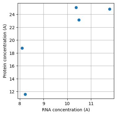
• We have a statistic called Pearson’s correlation coefficient, which has a value of 0.86.
• Since the value is larger than 0, we can say that the experimental results support the hypothesis that the RNA and protein expression levels of Protein A are positively correlated.

Random Incidences

• However, we need to consider whether our interpretation is valid.
• To test this, we will generate the same statistic using two independent variables, repeating this process five times.
• We found 3 out of 5 random association had a Pearson correlation coefficient (PCC) greater than 0.
• Therefore, observing a PCC greater than 0 might be too loose a criteria.

for i in range(5):
    rvs = generate_random_values_B()
    print(calculate_correlation(rvs)[0])   

0.5148158483005283
-0.6822188844235954
0.43813562081717283
-0.2495326763997526
0.10300182994047037

Statistical Inference

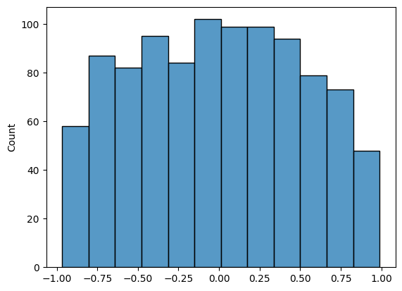
• Let’s generate more random numbers and calculate PCC multiple times.
• We repated this process 1000 times, obtaining a distribution of PCC values.
• Among these, 30 instances had a PCC greater than 0.85, representing 3% of the cases (30/1000 = 3%).
• In other words, we can observer a PCC larger than 0.85 in 3% of the experiments, even when the two variables are not correlated.

rhos= []
cnt = 0 
for i in range(1000):
    rvs = generate_random_values_B()
    rhos.append(calculate_correlation(rvs)[0]) 
    if calculate_correlation(rvs)[0] > 0.85:
        cnt += 1

sns.histplot(rhos)
print(cnt)

P-value

• We can calculate the probability of observing a statistic when the two variables are not correlated.
• The probability is called the p-value.
• We can estimate the p-value through simulation, as demonstrated above.
• However, in certain cases, we can calculate the p-value exactly.
• In other words, p-values can often be calculated quickly without the need for simulation.
• Pearson’s correlation coefficient is one such statistic with a well defined distribution, allowing us to calculate the p-value accurately.
• You can calculate PCC using stats.pearsonr function of scipy package.

Statistical inference

• Now, we can make a statistical inference using the p-value.
• Typically, we set a cutoff for the p-value, with 0.05 or 5% being the most commonly used threshold.
• If the p-value of a statisic for an observation is less than 5%, we call the observation statistically significant, as it is unlikely (less than 5% probability) to have occurred by chance.